Parameter estimates for regression: least squares, gradient descent and monte carlo methods22/8/2015
[data and R code for this post are available on github]
In this post I will cover three ways to estimate parameters for regression models; least squares, gradient descent and Monte Carlo methods. The aim is to introduce important methods widely used in machine learning, such as gradient descent and Monte Carlo, by linking them to a common "use case" in the different data science communities, such as linear regression. Regression is one of the first prediction methods invented, and the three approaches I will be discussing, are typically used by three different communities. Least squares is probably the most common method, mainly employed by frequentist statisticians and also used as the default method for many easy to use packages in R or Python (e.g. the lm function in R). Gradient descent is the machine learning approach to the problem. My favorite resource on the topic is the famous machine learning course by Andrew Ng on Coursera. In machine learning, the overall approach to problem solving and prediction is rather different compared to more classical statistics, even though it heavily relies on statistics (check out this answer by Sebastian Raschka on the origins of machine learning, I think it makes my point clear). I think one of the reasons why Andrew Ng uses gradient descent in the first place, instead of other methods like the least squares, is probably that he wants to stress the importance of the method in the machine learning community. By using gradient descent, he highlights how in machine learning it's often more important to approximate a solution by defining an iterative procedure able to efficiently explore the parameter space, instead of obtaining an exact analytical solution. Finally, there is the Bayesian way of doing things. Monte Carlo methods are powerful tools to explore the parameter's space and obtain the full posterior distribution, instead of just point estimates. This is something that requires a bit more introduction and explanation, and while I tried to do so in the remaining of this blog post, this is certainly far from being a comprehensive resource on Bayesian modeling. For the ones that want to dig deeper into regression and Bayesian approaches I would suggest reading Gelman's book on hierarchical modeling, one of my favorite resources in the field.
least squares regression
Least squares regression is the oldest method, dating back to Gauss (end of the 18th century). In the classical model, we have:
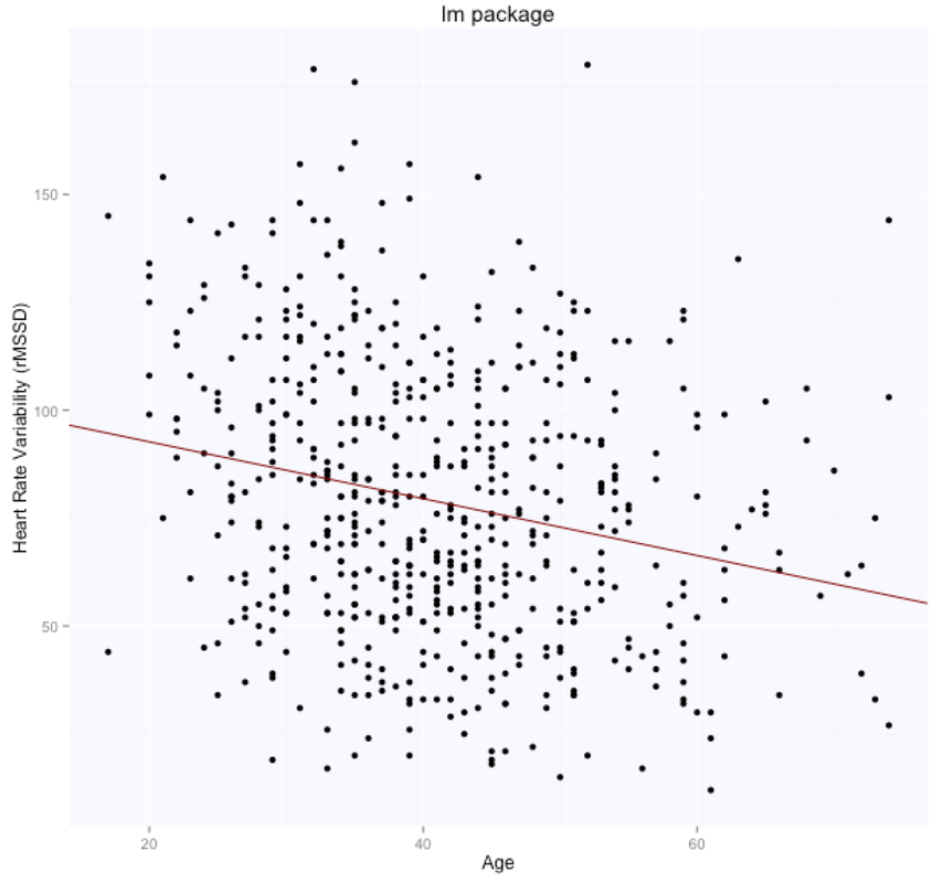
\[ y_i = X_i \beta + \epsilon_i \] where $y$ - the outcome variable -, and $\epsilon$ are vectors of $n$ elements, $X$ is a matrix with $n$ rows - the samples - and $k$ columns - the predictors. $\beta$ is a vector of length $k$, with one element per predictor. The regression problem, starting from a set of predictors $X$ and an outcome variable $y$, concerns in finding the $\hat{\beta}$ minimizing the sum of squared residuals. As residuals, we mean $r_i = y_i - X_i \hat{\beta}$, that are different from the errors $\epsilon_i = y_i - X_i \beta$. Basically, the sum of squared residuals is a way to quantify the accuracy of our prediction model. Since we have an outcome variable, we can determine how well our model (i.e. the parameters $\hat{\beta}$) can predict the outcome variable, based on our predictors, by computing: \[ sum\:of\:squares = \sum_{i=1}^n (y_i - X_i \hat{\beta})^2 \] What we want to achieve, is to find the $\hat{\beta}$ that makes the sum of the values $(y_i - X_i \hat{\beta})^2$ the smallest possible given our data. The solution to this problem, in matrix notation, is the following: \[ \hat{\beta} = (X^t X)^{-1}X^ty \] Here is the R code in closed form as well as using the lm package:
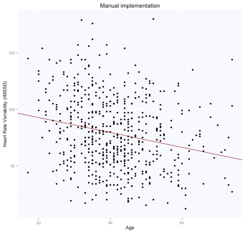
For the manual implementation of the least squares in closed form solution, we first add the intercept (an array of 1s) and then solve according to the formula above.
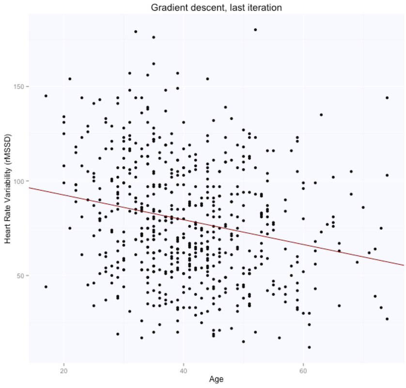
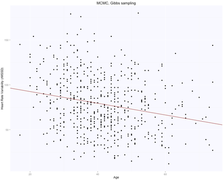
The solution is, as expected, exactly the same for both methods (matrix form and using the lm package), with intercept $105.86$ (supposedly the HRV of a newborn), and slope $-0.65$, i.e. according to this model we loose one ms in rMSSD every year. Note that lm takes care of adding the intercept for us, and we need to specify only the age parameter. Here are the data and the regression line:
This implementation seemed simple enough, and since it is provided by most standard packages, the temptation could be to stop here. However, there are very valid reasons to learn both gradient descent and Monte Carlo methods.
First of all, problems are typically not this simple. For most non-linear regression problems, there is no closed form solution. Also, the closed form solution scales very poorly when we have much more data, especially in terms of parameters. So, in general, it would be better to have a simple approach to solve optimization problems in a more generic way. Secondly, gradient descent is not only an alternative to least squares for parameter estimation, but most importantly it is one of the algorithms at the foundations of machine learning. As such, gradient descent is an important algorithm to learn, that will occur many times while using other methods, beyond linear regression (e.g. neural networks). Finally, when it comes to Monte Carlo methods, an entire new world opens up due to the flexibility of using Bayesian modeling and probabilistic graphical models to model relations between variables and perform inference on the parameters of interest. However, many of these models are often analytically intractable, and here is where Monte Carlo methods come into play. For such complex models we typically do not write our own samplers (i.e. our own tools to estimate the parameters), but rely on tools such as JAGS in R or PyMC in Python. However, it can be useful to understand how Monte Carlo methods work in the context of a simple linear regression example. gradient descent
Gradient descent is one of the core components of machine learning. For this implementation, I will use the notation and terminology used by Andrew Ng in his course. First, we define our hypothesis function, which is nothing different from our regression equation in the least squares example:
\[ h_{\theta}(x) = \theta_0 + \theta_1 x \] Here our $\beta$ parameters have been replaced by $\theta$, but the problem is exactly the same as before. Even the idea behind our gradient descent algorithm is basically the same as before, i.e. to minimize the sum of squared errors. This time, we call the function to minimize the cost function: \[ J(\theta_0, \theta_1) = \frac{1}{2m} \sum_{i=1}^m (h_0(x^{(i)}) - y^{(i)} )^2 \] Why do we talk about an hypothesis and cost function this time? Here we think about the problem differently. We make an hypothesis about the parameters values, assigning values to $\theta_0$ and $\theta_1$, and then evaluate how good our hypothesis is, by computing the cost function. Then, we optimize the parameters values iteratively. This optimization is what the gradient descent algorithm does. Why do we need it? Simply put, we need an efficient way to explore the parameter's space, especially when we have many parameters, and find the optimal values quickly. To minimize the cost function, we set the derivative with respect to $\theta$ to zero. As very well explained by Andrew Ng, who also provides great graphical representations of the intuition behind gradient descent, by taking the derivative, i.e. the line tangent to the cost function, we obtain a direction towards the which we can move to minimize the cost function. The only other additional parameter is the learning rate, $\alpha$, which controls how big our steps towards the minimum are. So, the generic gradient descent equation is defined as: \[ \theta_j := \theta_j - \alpha \frac{\partial}{\partial \theta_j} J(\theta_0, \theta_1) \] Replacing our equations and computing the derivative for our linear regression problem (while skipping the math): \[ \theta_0 := \theta_0 - \alpha \frac{1}{m} \sum_{i=1}^m (h_{\theta}(x^{(i)}) - y^{(i)} ) \]
\[
\theta_1 := \theta_1 - \alpha \frac{1}{m} \sum_{i=1}^m (h_{\theta}(x^{(i)}) - y^{(i)} ) x^{(i)} \]
The two equations are repeated until convergence, so we start with random values and then iteratively improve them. Convergence means that the gradient descent is sufficiently close to a stationary point, i.e. a local or global minimum. For linear regression, the cost function will always be convex, which means we will always reach a global minimum and won't get stuck in local minimum. Here is the R code for estimating the parameters of our regression model using gradient descent:
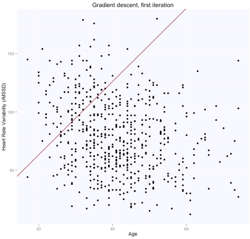
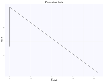
The cost function was first used to determine our partial derivatives and in this script it's now used only to track progress. Let's look at our theta estimates at the first and last iteration:
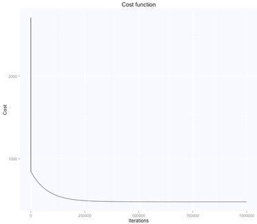
The gradient descent algorithm learnt the parameters theta (figure above on the right, while starting from random $\theta$ values, shown in the figure above on the left), which are now very similar to what we had with the beta's before. $\theta_0$ is $105.7$, while $\theta_1$ is $-0.66$. Here are the evolution of the parameters space and the cost function:
The optimal value (lowest cost) for the parameters theta is the one in the bottom right corner of the left figure above. The point corresponds to the lowest cost computed with our cost function. The evolution of all these parameters is logged in the history variable in the script above.
monte carlo methods
The first two methods, least squares and gradient descent, were rather easy to introduce and understand. While there is a lot more to them, the principle behind their use is quite straightforward. For the least squares, we simply find an analytical solution to our problem. Not always applicable, but good enough in many situations. For the gradient descent, we have an optimization problem solved iteratively starting with random parameters values. The main reason for introducing gradient descent, was that it is widely used in machine learning and therefore important to understand for the ones working in the field. However, Monte Carlo methods require a bit more background.
quick intro to bayesian statistics
In Bayesian statistics we start from the following:
\[ p(\theta | y) = \frac{p(y | \theta)p(\theta) }{p(y)} \] where we call $p(y | \theta)$ the likelihood, $p(\theta)$ the prior and $p(\theta | y)$ the posterior (let's not worry about $p(y)$ now, since this parameter is independent of $\theta$ and we can often ignore it). A prior is a density or mass function (probability distribution) on the parameter expressing our belief about those parameters. The likelihood is the component that depends on the data, and the factor by which our prior beliefs are updated to produce conclusions once we've seen some data. All inferences are performed on the distribution of the parameter given the data $p(\theta | y)$, called the posterior, our main variable of interest. parameter estimates in bayesian statistics
If the goal is to determine the parameters $\theta$ given a model (likelihood $p(y | \theta)$) and our prior beliefs $p(\theta)$, i.e. to determine the posterior $p(\theta | y)$, how do we go about it? We can proceed in different ways:
Due to the limitations of exact inference (not always applicable) and point estimates (we lack information about the full posterior distribution, and in certain cases, e.g. MLE, we might even overfit), we will only consider approximations and in particular Monte Carlo methods. monte carlo methods
Markov Chain Monte Carlo (MCMC) methods like Metropolis-Hastings or Gibbs sampling provide a way to approximate the value of an integral and we can use these methods to determine the posterior distribution when it is analytically intractable. MCMC techniques are often applied to solve integration and optimization problems in large dimensional spaces and there is a lot of theory here that should be covered, starting with Markov Chains, however, in this post I will just try to describe the general principle behind these methods and give an intuition of how they work.
Intuition MCMC methods assume that the prior distribution is specified by a function that can be easily evaluated at any point and that the value of the likelihood can also be computed for any value of $\theta$ and the data at hand. The method will produce an approximation of the posterior distribution in the form of a large number of samples of $\theta$ sampled from that distribution. So the basic idea is that even if we cannot compute the integral, we can evaluate it at any point. Then, we need a way to explore the parameters space so that the probability of being at a given point in the parameters space is proportional to the function we sample from (our so called target distribution, i.e. the posterior). This is why it works. By moving proportionally to the posterior distribution probabilities, the chain of samples we will eventually gather, will be representative of our $\theta$. To do so, we start at a random point and explore the parameter space using a proposal function. Since we start randomly, we typically discard those first samples (burn-in). The remaining component to put all of this together, is the proposal function. Let's see how this works for one of the most commonly used MCMC sampling algorithms, the Metropolis-Hastings algorithm. Metropolis-Hastings The Metropolis-Hastings algorithm requires that we can sample from our unnormalized posterior, i.e. the product of the prior and the likelihood, which we call the target distribution $\pi$. This is the case because of the acceptance rule used, which is a ratio of densities, and therefore we do not need to know the normalizing constant. The acceptance rule defines whether we make a move to the next location $x_j$, based on the proposal function evaluated in the current $x_i$ and next location $x_j$. While discussing the intuition, we stopped at the proposal function. So, what can we use as proposal function to decide where and when to move? The proposal can have different forms, we can consider for example a normal distribution, so that the proposed move will typically be near the current position. Using as proposal a normal, i.e. a symmetric distribution, makes things simpler because the acceptance rate for a new value $x_j$ from the current position $x_i$, is defined as: \[ a_{ij} = min(1, \frac{\pi(x_j)}{\pi(x_i)}) \] And therefore we only need to evaluate the target distribution at these two points (things are slightly more complicated with a non symmetrical proposal distribution, but I won't cover it here). By computing the value of the target distribution at $x_i$ and $x_j$ we decide if we want to make the move towards the new point. We always make the move if the value at the new point is higher. However, if the value is lower, we make the move only with probability $a_{ij}$. We'll see this later when we code the algorithm. We will use a uniform distribution between $0$ and $1$ to determine if we want to accept the new value and make the move when the value of the target distribution at $x_j$ is not higher than at $x_i$. After many steps we will obtain the target posterior distribution $\pi$. Now that we have some background on Bayesian statistics and MCMC, let's implement the Metropolis-Hasting algorithm for our univariate regression example. We first introduce our new notation. We assume independent normal distribution with mean $0$ and standard deviation $\sigma$ for $\epsilon$ and write the equation in compact form as: \[ y_i = X_{i} \beta + \epsilon_i, \quad \epsilon_i \sim N(0, \sigma^2), \quad i = 1, \dots, n \] Equivalently, we can express the relation between predictors and predicted variables as: \[ y_i \sim N( X_{i} \beta, \sigma^2), \quad i = 1, \dots, n \] Which is form I typically use, and one of the notations you'll find in Gelman's books.
Normally, especially for more complex models, we don't write our own sampler but we use software packages that do that for us. All we do is to specify the model's parameter, the likelihood and prior, and let the software packages do the sampling (more on this later). However, first it is as usual very useful to implement a small sampler to understand better how the whole thing works, in a simple example (acceptance, proposal function, etc). Then, we'll do the same using one of these software packages. Here is the code to estimate the parameters using the Metropolis-Hastings algorithm, which borrows a lot from here:
In the code above, after defining our likelihood, prior and posterior, we implemented the Metropolis-Hastings algorithm using a normal distribution as proposal function. This choice implies that we simply compute our posterior in the current and proposed point in order to determine the acceptance rate and decide if we are going to make the move or not. Once we computed the acceptance, we use R's runif function to decide if we are moving to the next location or staying. In the long run, we will be exploring the parameters space with probability acceptance, which is exactly what we want. Note that we are summing over the likelihood and priors because we are taking the logarithms of the values. This is necessary because otherwise we will have numerical issues due to the tiny values we are trying to multiply.
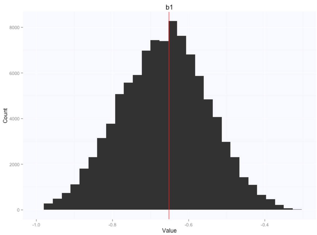
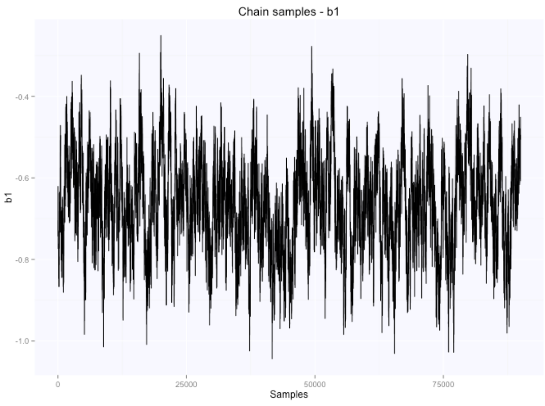
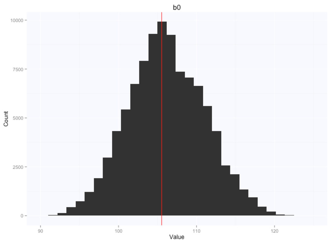
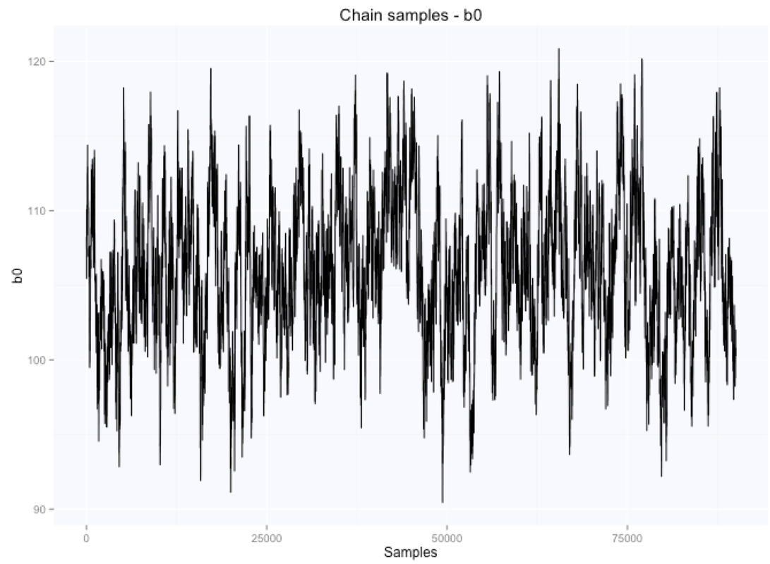
Let's look at the parameters estimates for the slope and intercept:
If we summarize the parameters posterior distributions using the mean of the samples extracted from our chain, we get $105.9$ for the intercept, and $-0.66$ for the slope.
We obtained almost the same results we had before using least squares or gradient descent, however this seemed a lot of extra complexity, even for the simple case of univariate regression. As I was saying above we typically use software packages that can do the sampling for us. What this means is that we need to worry only about specifying the likelihood and priors, and nothing else. Some of the most commonly used software packages are JAGS for R, STAN (created by Gelman) and PyMC for Python. I will be using JAGS. JAGS stands for Just Another Gibbs Sampler, and as the name states, uses a sampling technique called Gibbs sampling, which is slightly different from the Metropolis-Hastings algorithm we just implemented. Gibbs sampling Gibbs sampling can be seen as a special case of the Metropolis-Hastings algorithm, which is not always applicable, but has some advantages. For example, one of the main limitations of the Metropolis-Hastings algorithm is that we need to take good care of choosing the proposal distribution. If the proposal distribution is too narrow and the target distribution very spread out, it will not work well. On the other hand, Gibbs sampling does not require tuning of a proposal distribution. In Gibbs sampling, a proposed move affects only one parameter at a time, and the proposed move is never rejected. The main catch is that we must be able to generate samples from the posterior distribution conditioned on each individual parameter. Hopefully we gained an understanding of sampling methods from the previous section, and without entering in the details of the Gibbs sampler, we can have a look at how things work in JAGS. In general, it can be very hard to either define the proper proposal function (in case we use Metropolis-Hastings) or specify all the conditional distributions (in case we use Gibbs sampling), especially when we work in a high dimensional parameter space. Thus, we rely on software packages that do the job for us, and focus on specifying the model and priors only. Here is the JAGS code for univariate regression:
From the code above, we can see we specify our regression model similarly to our notation above, as $y_i \sim N( X_{i} \beta, \sigma^2)$. However we split the model definition in two lines, first defining the probabilistic part $y_i \sim N( \mu, \sigma^2)$ and then the deterministic one $\mu_i = X_{i} \beta$. We need to specify the model this way otherwise JAGS does not work. Then, we specify our priors over the parameters, and we are basically done.
The last step is to call the sampler passing our data (outcome and predictors), and specifying a couple of parameters such as the number of iterations and the burn-in period:
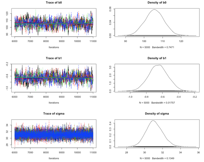
Here is the summary output using the Coda package (just call coda.samples instead of jags.samples, and then call plot(mcmc_samples)). We have four chains (the different colors) for the three parameters:
We can visually compare the posterior distributions for $\beta_0$ and $\beta_1$ to the ones obtained before using the Metropolis-Hastings algorithm, they look very similar.
Our results using JAGS and Gibbs sampling, are $105.6$ for the intercept and $-0.65$ for the slope, when taking the mean of the chains: summary
In this post I covered three ways to estimate parameters for regression models; least squares, gradient descent and Monte Carlo methods. The aim was to introduce important methods widely used in machine learning, such as gradient descent and Monte Carlo, by linking them to a use case which is widely used and understood by the different "data science" communities, such as linear regression.
We've seen, as expected, that regardless of the method (exact analytical solution or approximations), results are basically the same for this very simple univariate regression example. There are some clear advantages in using gradient descent or Monte Carlo methods with respect to least squares, such as better scalability or the derivation of the full posterior distribution. However, my main point here is that seeing how the same results can be obtained in many different ways and manually implementing most of these methods can be particularly useful to provide a unified perspective on a well known problem, such as regression, to the ones coming from different backgrounds and being used only to one approach or the other. For the ones interested in learning more about other ways in which the gradient descent algorithm is used to solve parameter optimization problems, I would suggest going through Andrew Ng machine learning course. In my work I got more and more interested in Bayesian modeling when I first approached hierarchical models. In addition to the conventional points in favor or Bayesian statistics, such as the full posterior distributions instead of point estimates and the use of priors (yes, they are a plus), the flexibility of hierarchical modeling in a Bayesian framework, allows to specify relations between variables very clearly. Especially for "small data" problems, generalized linear models and Bayesian inference provide a much better alternative to standard complete pooling or no-pooling models. By using probabilistic programming languages like JAGS, STAN or PyMC we can work on specifying the model and relations between variables and then let the sampler do the magic. For the ones interested in this topic and in seeing how hierarchical modeling can be used in many different applications to better model hierarchical relations that are very often encountered in real life applications (e.g. samples within people, cities within counties, etc.), I would suggest reading Data Analysis Using Regression and Multilevel/Hierarchical Models. For a lighter introduction, still showing the power of Bayesian modeling and hierarchical regression, start from this ipython notebook by Chris Fonnesbeck. Bayesian statistics is rather complex and obviously this post is far from being comprehensive. If all of this still seems very confusing, do as I did, go to London and visit Bayes' grave:
4 Comments
23/8/2015 11:26:26 pm
Nice post Marco. Seeing as you were using RMSSD HRV as a variable, we usually transform RMSSD using a natural log to make it more normally (Gaussian) distributed, and I wonder how normal the resulting distribution really is for large sample sizes?
Reply
Marco Altini
24/8/2015 12:30:35 am
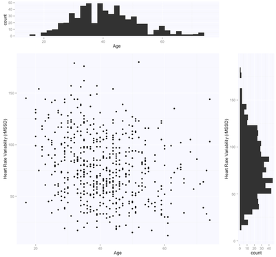
Thanks Simon. Indeed that's true, even though for this sample the data didn't seem particularly skewed for rMSSD (see very first figure, the histogram on the right), so I didn't transform it.
Reply
Hi Marco,
Reply
Marco Altini
7/10/2015 04:20:38 am
hi Daniel, thanks! Please feel free to go ahead and port the code. I've also been playing around more with python recently, looking forward to reading it!
Reply
Your comment will be posted after it is approved.
Leave a Reply. |
Marco ALtiniFounder of HRV4Training, Advisor @Oura , Guest Lecturer @VUamsterdam , Editor @ieeepervasive. PhD Data Science, 2x MSc: Sport Science, Computer Science Engineering. Runner Archives
May 2023
|

 RSS Feed